Vector¶

Authors:	Daniel Shiffman; Abhik Pal (p5 port)
Copyright:	This tutorial is adapted from The Nature of Code by Daniel Shiffman. This work is licensed under a Creative Commons Attribution-NonCommercial 3.0 Unported License. The tutorial was ported to p5 by Abhik Pal. If you see any errors or have comments, open an issue on either the p5 or Processing repositories.

The most basic building block for programming motion is the vector. And so this is where we begin. Now, the word vector can mean a lot of different things. Vector is the name of a new wave rock band formed in Sacramento, CA in the early 1980s. It’s the name of a breakfast cereal manufactured by Kellogg’s Canada. In the field of epidemiology, a vector is used to describe an organism that transmits infection from one host to another. In the C++ programming language, a Vector (std::vector) is an implementation of a dynamically resizable array data structure. While all interesting, these are not the definitions we are looking for. Rather, what we want is this vector:

A vector is a collection of values that describe relative position in space.

Vectors: You Complete Me¶

Before we get into vectors themselves, let’s look at a beginner Processing example that demonstrates why it is in the first place we should care. If you’ve read any of the introductory Processing textbooks or taken a class on programming with Processing (and hopefully you’ve done one of these things to help prepare you for this book), you probably, at one point or another, learned how to write a simple bouncing ball sketch.

from p5 import *
x = 100
y = 100

xspeed = 1
yspeed = 3.3

def setup():
    size(200, 200)
    background(255)

def draw():
    global x
    global y
    global xspeed
    global yspeed

    no_stroke()
    fill(255, 10)
    rect((0, 0), width, height)

    # add the current speed to the location
    x = x + xspeed
    y = y + yspeed

    if x > width or x < 0:
        xspeed = -xspeed

    if y > height or y < 0:
        yspeed = -yspeed

    stroke(0)
    fill(175)
    circle((x, y), 16)

if __name__ == '__main__':
    run()

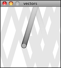
In the above example, we have a very simple world – a blank canvas with a circular shape (“ball”) traveling around. This “ball” has some properties.

LOCATION: x and y
SPEED: xspeed and yspeed

In a more advanced sketch, we could imagine this ball and world having many more properties:

ACCELERATION: xacceleration and yacceleration
TARGET LOCATION: xtarget and ytarget
WIND: xwind and ywind
FRICTION: xfriction and yfriction

It’s becoming more and more clear that for every singular concept in this world (wind, location, acceleration, etc.), we need two variables. And this is only a two-dimensional world, in a 3D world, we’d need x, y, z, xspeed, yspeed, zspeed, etc. Our first goal in this chapter is learn the fundamental concepts behind using vectors and rewrite this bouncing ball example. After all, wouldn’t it be nice if we could simple write our code like the following?

Instead of:

x = ...
y = ...
xspeed = ...
yspeed = ...

Wouldn’t it be nice to have…

location = Vector(...)
speed = Vector(...)

Vectors aren’t going to allow us to do anything new. Using vectors won’t suddenly make your Processing sketches magically simulate physics, however, they will simplify your code and provide a set of functions for common mathematical operations that happen over and over and over again while programming motion.

As an introduction to vectors, we’re going to live in 2 dimensions for quite some time (at least until we get through the first several chapters.) All of these examples can be fairly easily extended to three dimensions (and the class we will use – p5.Vector – allows for three dimensions.) However, for the time being, it’s easier to start with just two.

Vectors: What are they to us, the Processing programmer?¶

Technically speaking, the definition of a vector is the difference between two points. Consider how you might go about providing instructions to walk from one point to another.

Here are some vectors and possible translations:

You’ve probably done this before when programming motion. For every frame of animation (i.e. single cycle through Processing’s p5.draw() loop), you instruct each object on the screen to move a certain number of pixels horizontally and a certain number of pixels (vertically).

For a Processing programmer, we can now understand a vector as the instructions for moving a shape from point A to point B, an object’s “pixel velocity” so to speak. For every frame:

\[location = location + velocity\]

If velocity is a vector (the difference between two points), what is location? Is it a vector too? Technically, one might argue that location is not a vector, it’s not describing the change between two points, it’s simply describing a singular point in space – a location. And so conceptually, we think of a location as different: a single point rather than the difference between two points.

Nevertheless, another way to describe a location is as the path taken from the origin to reach that location. Hence, a location can be represented as the vector giving the difference between location and origin. Therefore, if we were to write code to describe a vector object, instead of creating separate Point and Vector classes, we can use a single class which is more convenient.

Let’s examine the underlying data for both location and velocity. In the bouncing ball example we had the following:

\[\begin{split}\begin{align*} location &\to \mathtt{x}, \mathtt{y} \\ velocity &\to \mathtt{xspeed}, \mathtt{yspeed} \end{align*}\end{split}\]

Notice how we are storing the same data for both – two numbers, an x and a y. If we were to write a vector class ourselves, we’d start with something rather basic:

class Vector:
    def __init__(self, x, y):
        self.x = x
        self.y = y

At its core, a p5.Vector() is just a convenient way to store two values (or three, as we’ll see in 3D examples.).

And so this…

x = 100
y = 100
xspeed = 1
yspeed = 3.3

…becomes…

location = Vector(100, 100)
velocity = Vector(1, 3.3)

Now that we have two vector objects (location and velocity), we’re ready to implement the algorithm for motion – location = location + velocity. In the bouncing ball example, without vectors, we had:

# add the current speed to the location
x = x + xspeed
y = y + yspeed

By default Python’s + operator works on primitive values, however we can teach Python to add two vectors together using the + operator. The p5.Vector class is implemented with functions for common mathematical operations using the usual operators(+ for addition, * for multiplication, etc) These allow us to rewrite the above as:

# add the current speed to the location
location = location + velocity

Vectors: Addition¶

Before we continue looking at the p5.Vector class and its p5.Vector.__add__() method (purely for the sake of learning since it’s already implemented for us in Processing itself), let’s examine vector addition using the notation found in math/physics textbooks.

Vectors are typically written as with either boldface type or with an arrow on top. For the purposes of this tutorial, to distinguish a vector from a scalar (scalar refers to a single value, such as integer or floating point), we’ll use an arrow on top:

Vector: \(\vec v\)

Scalar: \(x\)

Let’s say I have the following two vectors:

\[\begin{split}\vec u = \begin{pmatrix} 5 \\ 2 \end{pmatrix}, \qquad \vec v = \begin{pmatrix} 3 \\ 4 \end{pmatrix}\end{split}\]

Each vector has two components, an \(x\) and a \(y\). To add two vectors together we simply add both \(x\) ‘s and both \(y\) ‘s. In other words:

\[\vec w = \vec u + \vec v\]

translates to:

\[\begin{split}\begin{align*} w_x &= u_x + v_x \\ w_y &= u_y + v_y \end{align*}\end{split}\]

and therefore

\[\begin{split}\vec w = \begin{pmatrix} 8 \\ 6 \end{pmatrix}\end{split}\]

Now that we understand how to add two vectors together, we can look at how addition is implemented in the p5.Vector class itself. Let’s write a function called __add__ that takes as its argument another p5.Vector object.

class Vector:
    def __init__(self, x, y):
        self.x = x
        self.y = y

    # New! A function to add another Vector to this vector. Simply
    # add the x components and the y components together.
    def __add__(self, v):
        self.x = self.x + v.x
        self.y = self.y + v.y
        return self

Now that we can how __add__ is written inside of p5.Vector, we can return to the location + velocity algorithm with our bouncing ball example and implement vector addition:

# add the current speed to the location
location = location + velocity

And here we are, ready to successfully complete our first goal – rewrite the entire bouncing ball example using p5.Vector.

from p5 import *

class Vector:
    def __init__(self, x, y):
        self.x = x
        self.y = y

    def __add__(self, v):
        self.x = self.x + v.x
        self.y = self.y + v.y
        return self

location = Vector(100, 100)
velocity = Vector(1, 3.3)

def setup():
    size(200, 200)
    background(255)

def draw():
    global location
    global velocity

    no_stroke()
    fill(255, 10)
    rect((0, 0), width, height)

    # add the current speed to the location
    location = location + velocity

    # We still sometimes need to refer to the individual
    # components of a Vector and can do so using the dot syntax
    # (location.x, velocity.y, etc)
    if location.x > width or location.x < 0:
        velocity.x = -velocity.x

    if location.y > height or location.y < 0:
        velocity.y = -velocity.y

    # display circle at x location
    stroke(0)
    fill(175)
    circle((location.x, location.y), 16)

if __name__ == '__main__':
    run()

Now, you might feel somewhat disappointed. After all, this may initially appear to have made the code more complicated than the original version. While this is a perfectly reasonable and valid critique, it’s important to understand that we haven’t fully realized the power of programming with vectors just yet. Looking at a simple bouncing ball and only implementing vector addition is just the first step. As we move forward into looking at more a complex world of multiple objects and multiple forces (we’ll cover forces in the next chapter), the benefits of p5.Vector will become more apparent.

We should, however, make note of an important aspect of the above transition to programming with vectors. Even though we are using Vector objects to describe two values – the x and y of location and the x and y of velocity – we still often need to refer to the x and y components of each Vector individually. When we go to drawn an object, there is no means for us to say (using our own Vector class):

circle(location, 16)

The p5.circle() function does not understand the Vector class we’ve just written. However this functionality has been implemented in p5’s p5.Vector class. For our own class, we must dig into the Vector object and pull out the x and the y components using object oriented syntax.

circle((location.x, location.y), 16)

The same issue arises when it comes time to test if the circle has reached the edge of the window, and we need to access the individual components of both vectors: location and velocity.

if location.x > width or location.x < 0:
       velocity.x = -velocity.x

Vectors: More Algebra¶

Addition was really just the first step. There is a long list of common mathematical operations that are used with vectors when programming the motion of objects on the screen. Following is a comprehensive list of all of the mathematical operations available as functions in the p5.Vector class. We’ll then go through a few of the key ones now. As our examples get more and more sophisticated we’ll continue to reveal the details of these functions.

u + v – add vectors
u - v – subtract vectors
k * u – scale the vector with multiplication
u / k – scale the vector with division
p5.Vector.magnitude() – calculate the magnitude of a vector
p5.Vector.normalize() – normalize the vector to unit length of 1
p5.Vector.limit() – limit the magnitude of a vector
p5.Vector.angle() – the heading of a vector expressed as an angle
p5.Vector.distance() – the euclidean distance between two vectors (considered as points)
p5.Vector.angle_between() – find the angle between two vectors
p5.Vector.dot() – the dot product of two vectors
pt.Vector.cross() – the cross product of two vectors

Having already run through addition, let’s start with subtraction. This one’s not so bad, just take the plus sign from addition and replace it with a minus!

Vector subtraction:

\[\vec w = \vec u - \vec v\]

translates to:

\[\begin{split}\begin{align*} w_x &= u_x - v_x \\ w_y &= u_y - v_y \end{align*}\end{split}\]

and the function inside our Vector therefore looks like:

def __sub__(self, v):
    self.x = self.x - v.x
    self.y = self.y - v.y
    return self

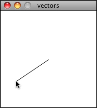
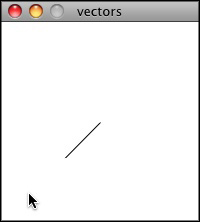
Following is an example that demonstrates vector subtraction by taking the difference between two points – the mouse location and the center of the window.

from p5 import *

class Vector:
    def __init__(self, x, y):
        self.x = x
        self.y = y

    def __add__(self, v):
        self.x = self.x + v.x
        self.y = self.y + v.y
        return self

    def __sub__(self, v):
        self.x = self.x - v.x
        self.y = self.y - v.y
        return self

def setup():
    size(200, 200)

def draw():
    background(255)

    # Two vectors, one for the moust location and one ofr the center
    # of the window
    mouse = Vector(mouse_x, mouse_y)
    center = Vector(width / 2, height / 2)

    # Vector subtraction!
    mouse = mouse - center

    # Draw a line to represent the vector
    translate(center.x, center.y)
    line((0, 0), (mouse.x, mouse.y))

if __name__ == '__main__':
    run()

Note

Both addition and subtraction with vectors follows the same algebraic rules as with real numbers.

The commutative rule: \(\vec u + \vec v = \vec v + \vec u\)
The associative rule: \(\vec u + (\vec v + \vec w) = (\vec u + \vec v) + \vec w\)

The fancy terminology and symbols aside, this is really quite a simple concept. We’re just saying that common sense properties of addition apply with vectors as well.

\[3 + 2 = 2 + 3\]

\[(3 + 2) + 1 = 3 + (2 + 1)\]

Moving onto multiplication, we have to think a little bit differently. When we talk about multiplying a vector what we usually mean is scaling a vector. Maybe we want a vector to be twice its size or one-third its size, etc. In this case, we are saying “Multiply a vector by 2” or “Multiply a vector by 1/3”. Note we are multiplying a vector by a scalar, a single number, not another vector.

To scale a vector by a single number, we multiply each component (x and y) by that number.

Vector multiplication:

\[\vec w = \vec v \cdot n\]

translates to:

\[\begin{split}\begin{align*} w_x &= v_x \cdot n \\ w_y &= v_y \cdot n \\ \end{align*}\end{split}\]

Let’s look at an example with vector notation.

\[\begin{split}\begin{align*} \vec u &= \begin{pmatrix} -3 \\ 7 \end{pmatrix}, \quad n = 3 \\ w &= u \cdot n \\ w_x &= -3 \cdot 3\\ w_y &= 7 \cdot 3\\ \vec w &= \begin{pmatrix} -9 \\ 21 \end{pmatrix} \end{align*}\end{split}\]

The function inside the Vector class therefore is written as:

def __mul__(self, n):
    # With multiplication, all components of a vector are
    # multiplied by a number
    self.x = self.x * n
    self.y = self.y * n
    return self

And implementing multiplication in code is as simple as:

u = Vector(-3, 7)

# this vector is now three times the size and is equal to (-9, 21)
u = u * 3

from p5 import *

class Vector:
    def __init__(self, x, y):
        self.x = x
        self.y = y

    def __add__(self, v):
        self.x = self.x + v.x
        self.y = self.y + v.y
        return self

    def __sub__(self, v):
        self.x = self.x - v.x
        self.y = self.y - v.y
        return self

    def __mul__(self, n):
        self.x = self.x * n
        self.y = self.y * n
        return self

def setup():
    size(200, 200)

def draw():
    background(255)

    mouse = Vector(mouse_x, mouse_y)
    center = Vector(width / 2, height / 2)
    mouse = mouse - center

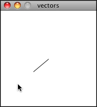
    # Vector multiplication!
    # The vector is now half its original size (multiplied by (1 / 2))
    mouse = mouse * (1 / 2)

    translate(center.x, center.y)
    line((0, 0), (mouse.x, mouse.y))

if __name__ == '__main__':
    run()

Division is exactly the same as multiplication, only of course using divide instead of multiply.

def __truediv__(self, n):
    self.x = self.x / n
    self.y = self.y / n
    return self

# ...

u = Vector(8, -4)
u = u / 2

Note

As with addition, basic algebraic rules of multiplication and division apply to vectors.

The associative rule: \((n \cdot m) \cdot \vec v = n \cdot (m \cdot \vec v)\)
The distributive rule, 2 scalars, 1 vector: \((n + m) \cdot \vec v = n \cdot \vec v + m \cdot \vec v\)
The distributive rule, 2 vectors, 1 scalar: \((\vec u + \vec v) \cdot n\)

Vectors: Magnitude¶

Multiplication and division, as we just saw, is a means by which the length of the vector can be changed without affecting direction. And so, perhaps you’re wondering: “Ok, so how do I know what the length of a vector is?” I know the components (x and y), but I don’t know how long (in pixels) that actual arrow is itself?!

The length or “magnitude” of a vector is often written as: \(\|\vec v\|\)

Understanding how to calculate the length (referred from here on out as magnitude) is incredibly useful and important.

Notice in the above diagram how when we draw a vector as an arrow and two components (x and y), we end up with a right triangle. The sides are the components and the hypotenuse is the arrow itself. We’re very lucky to have this right triangle, because once upon a time, a Greek mathematician named Pythagoras developed a nice formula to describe the relationship between the sides and hypotenuse of a right triangle.

The Pythagorean theorem: a squared plus b squared equals c squared.

Armed with this lovely formula, we can now compute the magnitude of as follows:

\[\|\vec v\| = \sqrt{v_x^2 + y_y^2}\]

or in Vector:

def mag(self):
    return sqrt(self.x * self.x + self.y + self.y)

from p5 import *

class Vector:
    def __init__(self, x, y):
        self.x = x
        self.y = y

    def __add__(self, v):
        self.x = self.x + v.x
        self.y = self.y + v.y
        return self

    def __sub__(self, v):
        self.x = self.x - v.x
        self.y = self.y - v.y
        return self

    def __mul__(self, n):
        self.x = self.x * n
        self.y = self.y * n
        return self

    def __div__(self, n):
        self.x = self.x / n
        self.y = self.y / n
        return self

    def mag(self):
        return sqrt(self.x * self.x + self.y * self.y)


def setup():
    size(200, 200)

def draw():
    background(255)

    mouse = Vector(mouse_x, mouse_y)
    center = Vector(width / 2, height / 2)
    mouse = mouse - center

    # The magnitude (i.e., the length) of a vector can be accessed by
    # the mag() function. Here it is used as the width of a rectangle
    # drawn at the top of the window.
    m = mouse.mag()
    fill(0)
    rect((0, 0), m, 10)

    translate(center.x, center.y)
    line((0, 0), (mouse.x, mouse.y))

if __name__ == '__main__':
    run()

Vectors: Normalizing¶

Calculating the magnitude of a vector is only the beginning. The magnitude function opens the door to many possibilities, the first of which is normalization. Normalizing refers to the process of making something “standard” or, well, “normal.” In the case of vectors, let’s assume for the moment that a standard vector has a length of one. To normalize a vector, therefore, is to take a vector of any length and, keeping it pointing in the same direction, change its length to one, turning it into what is referred to as a unit vector.

Being able to quickly access the unit vector is useful since it describes a vector’s direction without regard to length. For any given vector \(\vec u\), its unit vector (written as \(\hat u\)) is calculated as follows:

\[\hat u = \frac{\vec u}{\|\vec u\|}\]

In other words, to normalize a vector, simply divide each component by its magnitude. This makes pretty intuitive sense. Say a vector is of length 5. Well, 5 divided by 5 is 1. So looking at our right triangle, we then need to scale the hypotenuse down by dividing by 5. And so in that process the sides shrink, dividing by 5 as well.

In the Vector class, we therefore write our normalization function as follows:

def normalize(self):
    m = self.mag()
    self = self / m

Of course, there’s one small issue. What if the magnitude of the vector is zero? We can’t divide by zero! Some quick error checking will fix that right up:

def normalize(self):
    m = self.mag()
    if not (m == 0):
        self = self / m

from p5 import *

class Vector:
    def __init__(self, x, y):
        self.x = x
        self.y = y

    def __add__(self, v):
        self.x = self.x + v.x
        self.y = self.y + v.y
        return self

    def __sub__(self, v):
        self.x = self.x - v.x
        self.y = self.y - v.y
        return self

    def __mul__(self, n):
        self.x = self.x * n
        self.y = self.y * n
        return self

    def __truediv__(self, n):
        self.x = self.x / n
        self.y = self.y / n
        return self

    def mag(self):
        return sqrt(self.x * self.x + self.y * self.y)

    def normalize(self):
        m = self.mag()
        if not (m == 0):
            self = self / m


def setup():
    size(200, 200)

def draw():
    background(255)

    mouse = Vector(mouse_x, mouse_y)
    center = Vector(width / 2, height / 2)
    mouse = mouse - center

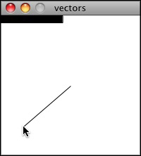
    # in this example, after the vector is normalized it is multiplied
    # by 50 so that it is viewable on screen. Note that no matter
    # where the mouse is, the vector will have the same length (50),
    # due to the normalization process
    mouse.normalize()
    mouse = mouse * 50

    translate(center.x, center.y)
    line((0, 0), (mouse.x, mouse.y))

if __name__ == '__main__':
    run()

Vectors: Motion¶

Why should we care? Yes, all this vector math stuff sounds like something we should know about, but why exactly? How will it actually help me write code? The truth of the matter is that we need to have some patience. The awesomeness of using the PVector class will take some time to fully come to light. This is quite common actually when first learning a new data structure. For example, when you first learn about an array, it might have seemed like much more work to use an array than to just have several variables to talk about multiple things. But that quickly breaks down when you need a hundred, or a thousand, or ten thousand things. The same can be true for Vector. What might seem like more work now will pay off later, and pay off quite nicely.

For now, however, we want to focus on simplicity. What does it mean to program motion using vectors? We’ve seen the beginning of this in this book’s first example: the bouncing ball. An object on screen has a location (where it is at any given moment) as well as a velocity (instructions for how it should move from one moment to the next). Velocity gets added to location:

location = location + velocity

And then we draw the object at that location:

circle((location.x, location.y), 16)

This is Motion 101.

Add velocity to location
Draw object at location

In the bouncing ball example, all of this code happened in Processing’s main tab, within p5.setup() and p5.draw() What we want to do now is move towards encapsulating all of the logic for motion inside of a class this way we can create a foundation for programming moving objects in Processing. We’ll take a quick moment to review the basics of object-oriented programming in this context now, but this book will otherwise assume knowledge of working with objects (which will be necessary for just about every example from this point forward). However, if you need a further refresher, I encourage you to check out the OOP Tutorial

The driving principle behind object-oriented programming is the bringing together of data and functionality. Take the prototypical OOP example: a car. A car has data – color, size, speed, etc. A car has functionality – drive(), turn(), stop(), etc. A car class brings all that stuff together in a template from which car instances, i.e. objects, are made. The benefit is nicely organized code that makes sense when you read it.

c = Car(red, big, fast)
c.drive()
c.turn()
c.stop()

In our case, we’re going to create a generic “Mover” class, a class to describe a shape moving about the screen. And so we must consider the following two questions:

What data does a Mover have?
What functionality does a Mover have?

Our “Motion 101” algorithm tells us the answers to these questions. The data an object has is its location and its velocity, two p5.Vector objects.

class Mover:
    def __init__(self, ...):
        self.location = Vector(...)
        self.velocity = Vector(...)

Note

To keep our code concise, we’re now switching to the p5.Vector class that comes with p5. So we can remove the custom Vector code that we wrote from our main sketch.

Its functionality is just about as simple. It needs to move and it needs to be seen. We’ll implement these as functions named update() and display(). update() is where we’ll put all of our motion logic code and display() is where we will draw the object.

def update(self):
    self.location = self.location + self.velocity

def display(self):
    stroke(0)
    fill(175)
    circle(self.location, 16)

We’ve forgotten one crucial item, however, the object’s constructor . The constructor is a special function inside of a class that creates the instance of the object itself. It is where you give the instructions on how to set up the object. In Python this constructor should always be called __init__. It gets called whenever we create a new object using my_car = Car().

Important

All methods defined in a class in Python require self as the first parameter.

In our case, let’s just initialize our mover object by giving it a random location and a random velocity.

class Mover:
    def __init__(self, width, height):
        self.location = Vector(random_uniform(width),
                               random_uniform(height))

        self.velocity = Vector(random_uniform(low=-2, high=2),
                               random_uniform(low=-2, high=2))

Let’s finish off the Mover class by incorporating a function to determine what the object should do when it reaches the edge of the window. For now let’s do something simple, and just have it wrap around the edges.

def check_edges(self):
    if self.location.x > width:
        self.location.x = 0

    if self.location.x < 0:
        self.location.x = width

    if self.location.y > height:
        self.location.y = 0

    if self.location.y < 0:
        self.location.y = height

Now that the Mover class is finished, we can then look at what we need to do in our main program. We first declare a placeholder for a Mover object:

mover = None

Then initialize the mover in p5.setup():

mover = Mover(width, height)

and call the appropriate functions in draw():

mover.update()
mover.check_edges()
mover.display()

Here is the entire example for reference:

from p5 import *

mover = None

class Mover:
    def __init__(self):
        # our object has two Vectors: location and velocity
        self.location = Vector(random_uniform(width),
                               random_uniform(height))

        self.velocity = Vector(random_uniform(low=-2, high=2),
                               random_uniform(low=-2, high=2))

    def update(self):
        # Motion 101: Locations change by velocity
        self.location = self.location + self.velocity

    def display(self):
        stroke(0)
        fill(175)
        circle(self.location, 16)

    def check_edges(self):
        if self.location.x > width:
            self.location.x = 0

        if self.location.x < 0:
            self.location.x = width

        if self.location.y > height:
            self.location.y = 0

        if self.location.y < 0:
            self.location.y = height

def setup():
    global mover
    size(200, 200)
    background(255)

    # make the mover object
    mover = Mover()

def draw():
    no_stroke()
    fill(255, 10)
    rect((0, 0), width, height)

    # call functions on Mover object
    mover.update()
    mover.check_edges()
    mover.display()

if __name__ == '__main__':
    run()

Ok, at this point, we should feel comfortable with two things – (1) What is a p5.Vector? and (2) How do we use Vectors inside of an object to keep track of its location and movement? This is an excellent first step and deserves an mild round of applause. For standing ovations and screaming fans, however, we need to make one more, somewhat larger, step forward. After all, watching the Motion 101 example is fairly boring – the circle never speeds up, never slows down, and never turns. For more interesting motion, for motion that appears in the real world around us, we need to add one more Vector to our class – acceleration.

The strict definition of acceleration that we are using here is: the rate of change of velocity. Let’s think about that definition for a moment. Is this a new concept? Not really. Velocity is defined as: the rate of change of location. In essence, we are developing a “trickle down” effect. Acceleration affects velocity which in turn affects location (for some brief foreshadowing, this point will become even more crucial in the next chapter when we see how forces affect acceleration which affects velocity which affects location.) In code, this reads like this:

velocity = velocity + acceleration
location = location + velocity

As an exercise, from this point forward, let’s make a rule for ourselves. Let’s write every example in the rest of this book without ever touching the value of velocity and location (except to initialize them). In other words, our goal now for programming motion is as follows – come up with an algorithm for how we calculate acceleration and let the trickle down effect work its magic. And so we need to come up with some ways to calculate acceleration:

ACCELERATION ALGORITHMS!

Make up a constant acceleration
A totally random acceleration
Perlin noise acceleration
Acceleration towards the mouse

Number one, though not particularly interesting, is the simplest, and will help us get started incorporating acceleration into our code. The first thing we need to do is add another p5.Vector to the Mover class:

class Mover:
    def __init__(self):
        location = Vector(...)
        velocity = Vector(...)

        # A new Vector for acceleration
        acceleration = Vector(...)

And incorporate acceleration into the update() function:

def update(self):
    # our motion algorithm is now two lines of code:
    self.velocity = self.velocity + self.acceleration
    self.location = self.location + self.velocity

We’re almost done. The only missing piece is the actual initialization in the constructor.

Let’s start the object in the middle of the window..

self.location = Vector(width / 2, height / 2)

…with an initial velocity of zero.

self.velocity = Vector(0, 0)

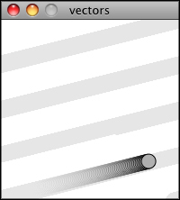
This means that when the sketch starts, the object is at rest. We don’t have to worry about velocity anymore as we are controlling the object’s motion entirely with acceleration. Speaking of which, according to “algorithm #1” our first sketch involves constant acceleration. So let’s pick a value.

self.acceleration = Vector(-0.001, 0.01)

Are you thinking – “Gosh, those values seem awfully small!” Yes, that’s right, they are quite tiny. It’s important to realize that our acceleration values (measured in pixels) accumulate into the velocity over time, about thirty times per second depending on our sketch’s frame rate. And so to keep the magnitude of the velocity vector within a reasonable range, our acceleration values should remain quite small. We can also help this cause by incorporating the Vector function p5.Vector.limit()

# the limit() function constrains the magnitude of the vector
self.velocity.limit(10)

This translates to the following:

What is the magnitude of velocity? If it’s less than 10, no worries, just leave it whatever it is. If it’s more than 10, however, shrink it down to 10!

Let’s take a look at the changes to the Mover class now, complete with acceleration and limit().

class Mover:
    def __init__(self):
        self.location = Vector(width / 2, height / 2)
        self.velocity = Vector(0, 0)

        # Acceleration is the key!
        self.acceleration = Vector(-0.001, 0.01)

        # this will limit the magnitude of velocity
        self.top_speed = 10

    def update(self):
        self.velocity = self.velocity + self.acceleration
        self.velocity.limit(self.top_speed)
        self.location = self.location + self.velocity

    # rest of the methods are the same

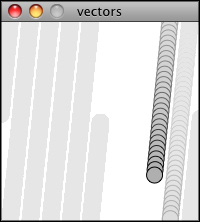
Ok, algorithm #2 – “a totally random acceleration.” In this case, instead of initializing acceleration in the object’s constructor we want to pick a new acceleration each cycle, i.e. each time update() is called.

def update(self):
    acc_x = random_uniform(low=(-1), high=1)
    acc_y = random_uniform(low=(-1), high=1)
    self.acceleration = Vector(acc_x, acc_y)
    self.acceleration.normalize()

    self.velocity = self.velocity + self.acceleration
    self.velocity.limit(self.top_speed)
    self.location = self.location + self.velocity

While normalizing acceleration is not entirely necessary, it does prove useful as it standardizing the magnitude of the vector, allowing us to try different things, such as:

scaling the acceleration to a constant value

acc_x = random_uniform(low=(-1), high=1)
acc_y = random_uniform(low=(-1), high=1)
self.acceleration = Vector(acc_x, acc_y)
self.acceleration.normalize()

self.acceleration = self.acceleration * 0.5

scaling the acceleration to a random value

acc_x = random_uniform(low=(-1), high=1)
acc_y = random_uniform(low=(-1), high=1)
self.acceleration = Vector(acc_x, acc_y)
self.acceleration.normalize()

self.acceleration = self.acceleration * random_uniform(2)

While this may seem like an obvious point, it’s crucial to understand that acceleration does not merely refer to the speeding up or slowing down of a moving object, but rather any change in velocity, either magnitude or direction. Acceleration is used to steer an object, and it is the foundation of learning to program an object that make decisions about how to move about the screen.

Vectors: Interactivity¶

Ok, to finish out this tutorial, let’s try something a bit more complex and a great deal more useful. Let’s dynamically calculate an object’s acceleration according to a rule, acceleration algorithm #4 – “the object accelerates towards the mouse.”

Anytime we want to calculate a vector based on a rule/formula, we need to compute two things: magnitude and direction. Let’s start with direction. We know the acceleration vector should point from the object’s location towards the mouse location. Let’s say the object is located at the point (x, y) and the mouse at (mouse_x, mouse_y).

As illustrated in the above diagram, we see that we can get a vector (dx, dy) by subtracting the object’s location from the mouse’s location. After all, this is precisely where we started this chapter – the definition of a vector is “the difference between two points in space!”

dx = mouse_x - x
dy = mouse_y - y

Let’s rewrite the above using Vector syntax. Assuming we are in the Mover class and thus have access to the object’s location Vector, we then have:

  mouse = Vector(mouse_x, mouse_y)
  direction = mouse - self.location


We now have a Vector that points from the mover's location all the
way to the mouse. If the object were to actually accelerate using
that vector, it would instantaneously appear at the mouse location.
This does not make for good animation, of course, and what we want to
do is now decide how fast that object should accelerate towards the
mouse.

In order to set the magnitude (whatever it may be) of our acceleration PVector, we must first ________ that direction vector. That’s right, you said it. Normalize. If we can shrink the vector down to its unit vector (of length one) then we have a vector that tells us the direction and can easily be scaled to any value. One multiplied by anything equals anything.

anything = ???
direction.normalize()
direction = direction * anything

To summarize, we have the following steps:

Calculate a vector that points from the object to the target location (mouse).
Normalize that vector (reducing its length to 1)
Scale that vector to an appropriate value (by multiplying it by some value)
Assign that vector to acceleration

And here are those steps in the update() function itself:

def update(self):
    mouse = Vector(mouse_x, mouse_y)

    # Step 1. direction
    direction = mouse - self.location

    # Step 2: normalize
    direction.normalize()

    # Step 3: scale
    direction = direction * 0.5

    # Step 4: accelerate
    self.acceleration = direction;

    self.velocity = self.velocity + self.acceleration
    self.velocity.limit(self.top_speed)
    self.location = self.location + self.velocity

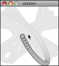
Note

Why doesn’t the circle stop when it reaches the target?

The object moving has no knowledge about trying to stop at a destination, it only knows where the destination is and tries to go there as fast as possible. Going as fast as possible means it will inevitably overshoot the location and have to turn around, again going as fast as possible towards the destination, overshooting it again, and so on, and so forth. Stay tuned for later chapters where we see how to program an object to “arrive”s at a location (slowing down on approach.)

Let’s take a look at what this example would look like with an array of Mover objects (rather than just one).

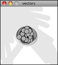
from p5 import *

num_movers = 20
movers = []

class Mover:
    def __init__(self):
        self.location = Vector(random_uniform(width),
                               random_uniform(height))

        self.velocity = Vector(0, 0)
        self.acceleration = Vector(0, 0)
        self.top_speed = 4

    def update(self):
        # our algorithm for calculating acceleration
        mouse = Vector(mouse_x, mouse_y)

        # find vector pointing towards the mouse
        direction = mouse - self.location

        # normalize
        direction.normalize()

        # scale
        direction = direction * 0.5

        # set acceleration
        self.acceleration = direction;

        self.velocity = self.velocity + self.acceleration
        self.velocity.limit(self.top_speed)
        self.location = self.location + self.velocity

    def display(self):
        stroke(0)
        fill(175)
        circle(self.location, 16)

    def check_edges(self):
        if self.location.x > width:
            self.location.x = 0

        if self.location.x < 0:
            self.location.x = width

        if self.location.y > height:
            self.location.y = 0

        if self.location.y < 0:
            self.location.y = height

def setup():
    size(200, 200)
    background(255)

    # creating many mover objects
    for _ in range(num_movers):
        movers.append(Mover())

def draw():
    no_stroke()
    fill(255, 10)
    rect((0, 0), width, height)

    # call functions on all objects in the array
    for mover in movers:
        mover.update()
        mover.check_edges()
        mover.display()

if __name__ == '__main__':
    run()